|
www.tlab.it
Co-occurrence
Toolkit
N.B.: Cette section est uniquement disponible en
anglais.
This tool, which can be used for a variety of
tasks, offers a set of techniques for building and analysing word co-occurrence matrices
with up to 5,000 columns.
The matrices to be built can be both symmetric and asymmetric, and they can represent the
co-occurrences of the words either within the whole corpus or within a subset of it.
N.B.: In the case of word co-occurrences, the
difference between symmetric and asymmetric matrices is that
symmetric matrices assume that the order of words does not matter
(i.e., they are represented as undirected graphs where the values
in a row and a column are the same), while asymmetric matrices take
into account the direction of co-occurrence and, for this reason,
are represented as directed graph where the values in a row (i.e.,
successor) and a column (i.e., predecessor) are not necessarily the
same.
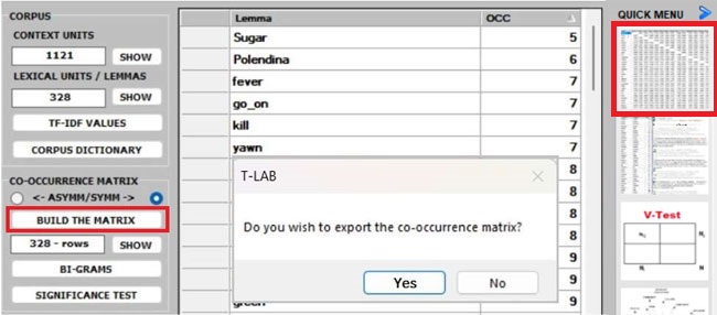
Whichever tool you are using, the way to export tables
and graphs is very simple (see picture below).
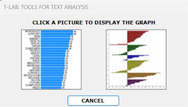
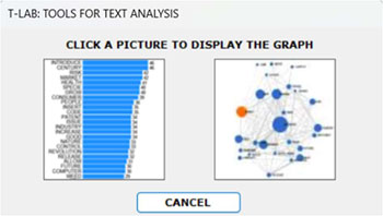
After building any co-occurrence matrix, the user
is allowed to extract the relevant information by using about
fifteen options listed on the left menu (see the above
picture).
N.B.:
- all the below pictures have been obtained by analysing the
English version of "The Adventures of Pinocchio" (by Carlo Collodi)
and its symmetric word co-occurrence matrix.
- all items in the tables are 'lemmas' because a T-LAB
lemmatization
has been performed on the Pinocchio corpus first.
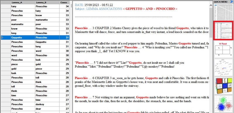
- whatever matrix you are analysing, it is always possible to check
the text segments in which pairs of words co-occur (see picture
below).
Below
are the descriptions of the various analysis options:
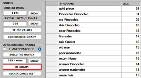
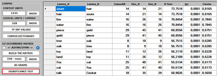
1 -Both the BI-GRAMS and the SIGNIFICANCE TEST extract pairs of words (e.g., collocations)
which can be relevant for customizing the corpus dictionary and also for
detecting small groups of related words which can affect any cluster analysis
(see pictures below).
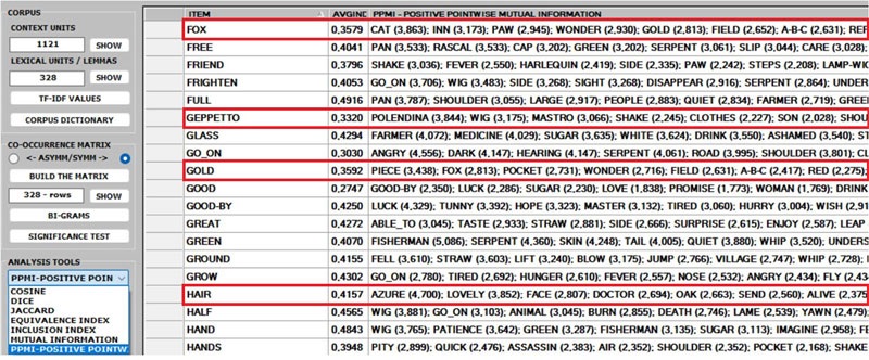
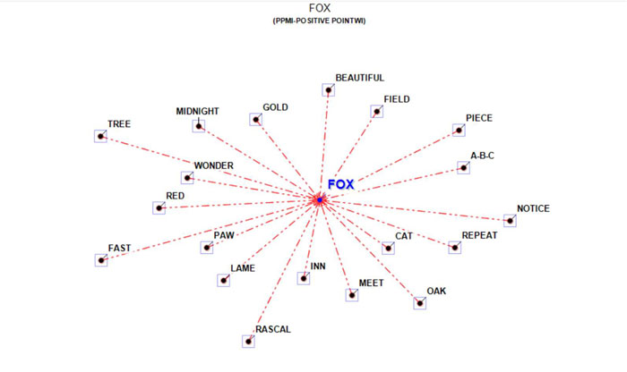
2 - The ASSOCIATIONS option, in addition to the
indexes used by other T-LAB
tools (see Associations and Co-Word Analysis), includes the PPMI (i.e., Positive Pointwise Mutual
Information), which is a measure of how much more likely two words
are to co-occur than by chance, based on their probabilities in a
text corpus. It can be used to distinguish between words that are
simply co-occurring by chance and words that are semantically
related. It can also reduce the effect of high-frequency words that
co-occur with many other words by chance. Moreover, unlike other
indexes (e.g., Cosine, Dice, Jaccard etc.) its maximum value is not
'1' and its upper bound can vary.
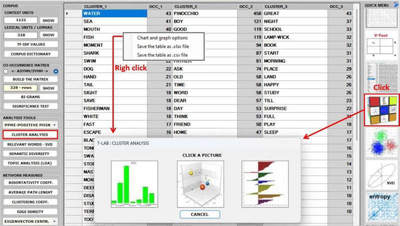
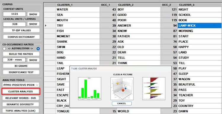
3 - The CLUSTER
ANALYSIS offers three methods for analysing a word
co-occurrence matrix: Hierarchical,
K-Means and Louvain.
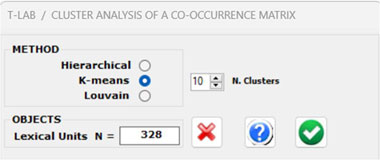
All the above three methods use vectors which are
normalized by the cosine coefficient, and one of them (i.e., the
K-Means) performs the clustering on the first 10 dimensions
obtained by a SVD (i.e.,
Singular Value Decomposition) of the normalized word co-occurrence
matrix.
To evaluate the quality of clustering results,
T-LAB provides the Silhouette scores for each data point.Moreover,
when clicking the ‘Q’ button
located at the bottom left corner of the screen, the user is
allowed to obtain three different quality indices (i.e.:
Calinski-Harabasz, Dunn and ICC-rho).
N.B.:
- Depending on the clustering method, the relationships between words within each cluster
can be visualized through different types of charts and graphs.
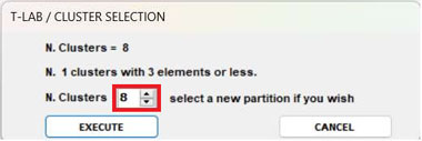
- When performing a hierarchical clustering, the user is allowed to
change the number of clusters (i.e., the cluster partition) within
a range from 3 to 20.
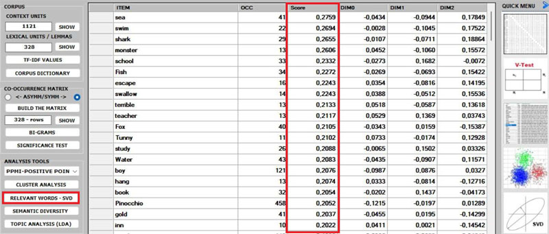
4 - The RELEVANT
WORDS - SVD provides a relevance score for each word,
which is computed by summing the square of its first 3 dimensions
(i.e., the eigenvectors), each one multiplied by its corresponding
singular value, and then by computing the square root of that
sum.
This means that the words with the higher scores are the farthest
from the point of origin, which is the point where the horizontal
axis (x-axis) and the vertical axis (y-axis) intersect. And, for
this reason, they are the words that most contribute to organizing
semantic polarizations, which can also have emotional
connotations.
N.B.: In this case, the SVD is performed on a centered matrix and
therefore it is equivalent to PCA (i.e., Principal Component
Analysis).
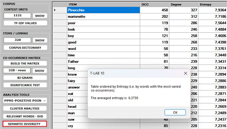
5 - The SEMANTIC
DIVERSITY of each word (i.e., its ability to have links
with many other words) is measured by means of the entropy index.
N.B.: The average entropy of the word co-occurrence
matrix can be used to quantify the 'complexity' of a text, since
more complex texts (i.e., texts in which many words cooccur with a
variety of other words) tend to have higher entropy than simpler
texts (i.e., texts in which many words cooccur with only a few
other words and - for that reason - are more predictable). And,
since high entropy corresponds to low predictability, it may be
also interesting to check which words in a text have higher
predictability values (i.e., low entropy).
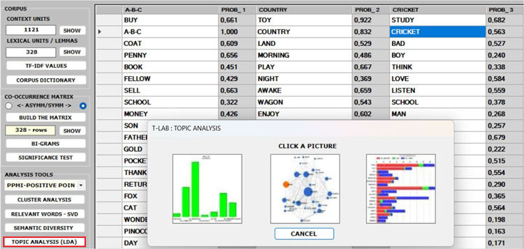
6 - The TOPIC
ANALYSIS of the word co-occurrence matrix uses the same
algorithm of the T-LAB Modeling of Emerging Themes tool (i.e., Latent
Dirichlet Allocation and the Gibbs Sampling); however, in this
case, both the indexes of the matrix (i.e., the 'i' and the 'j')
refer to the same words and the values correspond to their
co-occurrences. As can be verified, the results of this approach
are quite interesting and consistent.
N.B.: In the table below, the words are ordered by
their frequency within each topic.
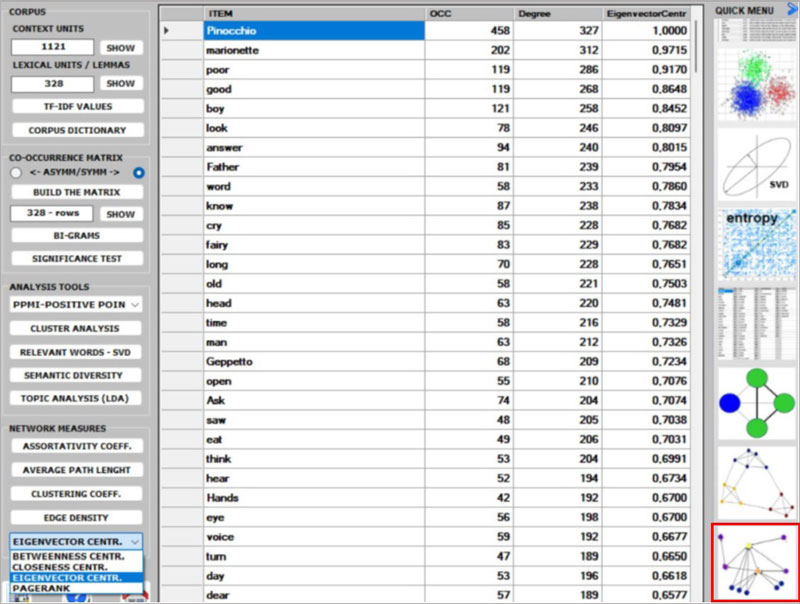
7 - Regarding the five CENTRALITY MEASURES (i.e., Betweenness
centrality, Closeness centrality, Eigenvector centrality, Katz
centrality and PageRank centrality) we observe that, especially in
the case of a symmetric word co-occurrence matrix, they are closely
related to each other. Moreover, they usually rank more highly the
words with higher occurrence values. The only exception seems to be
the Betweenness centrality. In fact, it is possible for a vertex to
have high betweenness centrality (i.e., to be able to connect
important parts of the network) without having high indegree or
high outdegree.
N.B.:
- All definitions of centrality measures, as well as their
algorithms, can be easily checked on Wikipedia.
- In T-LAB, all results of
centrality measures are normalized to the maximum value. This means
that all of the results are between 0 and 1, which makes them
easier to compare.
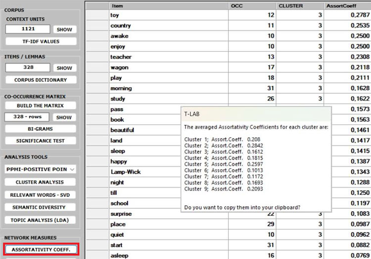
8 - The ASSORTATIVITY COEFFICIENT is a measure of how
likely nodes of a certain type are to be connected to other nodes
of the same type (i.e., 'similar' in some respects). In the case of
T-LAB, the types refer to the
results of a previous cluster analysis. Therefore, (a) if- for any
'i' node - the assortativity coefficient is positive and high, then
it indicates that the node is strongly connected with other nodes
of the same cluster; (b) if - for any 'k' cluster - the average
assortativity coefficient is positive and high, then it indicates
that the nodes which belong to the cluster are strongly connected
with each other; (c) a global average high positive assortativity
coefficient indicates that the clustering algorithm has
successfully grouped nodes based on their links within the cluster
they belong to. This means that nodes within the same cluster are
more likely to be connected to each other than nodes from different
clusters.
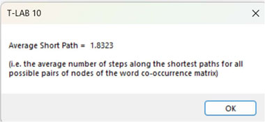
9 - The AVERAGE
PATH LENGTH (or average short path), in this case, is
defined as the average number of steps along the shortest paths for
all possible pairs of nodes of the word co-occurrence
matrix.
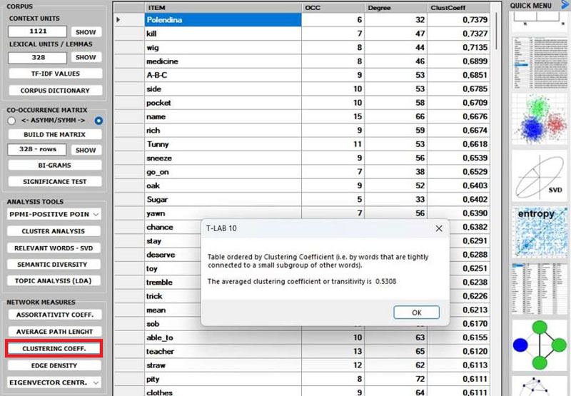
10 - The CLUSTERING
COEFFICIENT deserves special attention. In fact, the
'local' clustering coefficient is a measure of the degree to which
nodes in a graph tend to cluster together and to pair up with each
other (i.e., something like 'The friend of my friend is my
friend.'). In other words, the clustering coefficient of a node
(i.e., word) quantifies how close its neighbours (i.e., other
words) are to being a tightly connected subgroup (i.e., a clique).
It is computed as the proportion of the 'actual' connections among
its neighbours compared with the number of all its 'possible'
connections. Its maximum value is '1', and the average clustering
coefficient of all nodes it is also known as transitivity of the network.
N.B.: When a network has a large clustering
coefficient and a small average path length it can be considered a
'small world' (see Wikipedia).
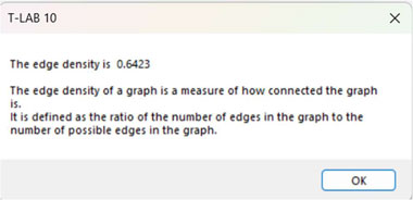
11 - The EDGE
DENSITY is a measure of how connected the graph is. It
is defined as the ratio of the actual number of edges in the graph
to the possible number of edges in the graph.
A high edge density indicates that the nodes in the graph are more
likely to be connected to each other. This means that there are
many paths between any two nodes in the graph. A low edge density
indicates that the nodes in the graph are more likely to be
disconnected from each other. This means that there are few paths
between any two nodes in the graph.
N.B.: It appears that there is a positive
correlation between edge density and clustering coefficient. In
fact, both measures refer to the connectivity of a graph and can be
used to compare the properties of different graphs (i.e., in this
case, the properties of different co-occurrence matrices).
.
|


