Word Associations

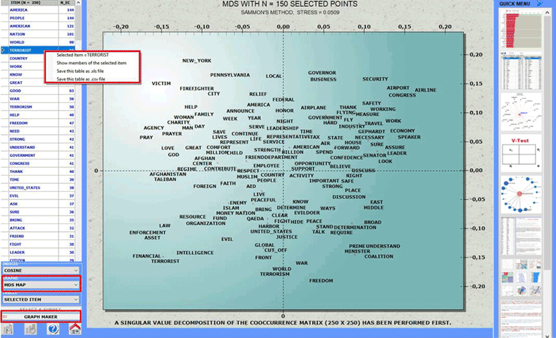
N.B.: The pictures shown in this section have been obtained by using a previous version of T-LAB. These pictures look slightly different in T-LAB 10. Also: a) there is a new option which allows the user to plot a MDS Map with the most relevant words; b) there is a new button (Graph Maker) which allows the user to create several dynamic charts in HTML format; c), by right clicking on the keyword tables , additional options become available; d) a quick access gallery of pictures which works as an additional menu allows one to switch between various outputs with a single click. Some of these new features are highlighted in the below image

This T-LAB tool allows us to pick out co-occurrence and similarity relationships which, within any corpus or its subset, determine the local meaning of selected key-terms.

Such a tool can be used with the default options (A) or through options selected by the user (B).

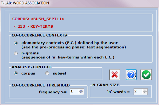
In the first case (A: default) word co-occurrences are computed within the elementary contexts (e.g. sentences, fragments, paragraphs). In the second one (B: options selected by the user) word co-occurrences can also be computed within n-grams (i.e. sequences of two or more words) and the user is also enabled to choose the minimum threshold of co-occurrences to be considered.

The working window (see below) is made available immediately after the computation of co-occurrences between all the words included in the list selected by the user has been done.

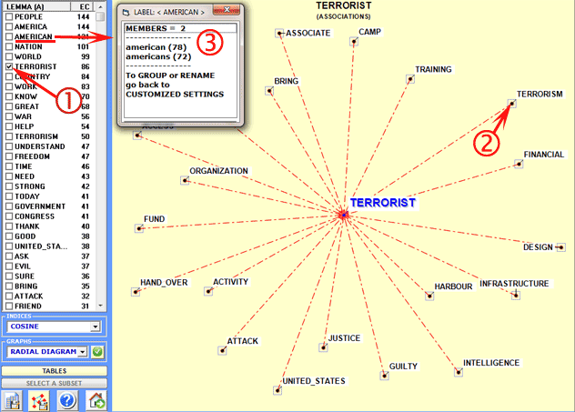
On the left of the above window there is a table with the key-term list and numerical values indicating the number of elementary contexts (EC) or n-grams where each key-term is present.

Either by clicking a item in the table (see '1' above) or by clicking on a point of the charts (see '2' above) it is possible to check the associations of each target word. Moreover, by clicking any item of the table (see '3' above') it is possible to check which words are included in the corresponding lemma or semantic class.

Each time the selection of associated words is carried out by the computation of an Association Index (see the corresponding item of the glossary) or by the computation of second order similarities (see the note at the end of this page). In the first case the available indexes are six (Cosine, Dice, Jaccard, Equivalence, Inclusion and Mutual Information) and their computation is quite fast. In the second case (i.e. second order similarities), as the computation requires lots of comparisons, it can take a number of minutes. Moreover the user has to take into account that the greater the number of words included in his list, the more reliable the similarity values become.

For each query, T-LAB produces graphs and tables. Both graphs and tables can be saved using the appropriate buttons.

In the radial diagrams the lemma selected is placed in the center. The others are distributed around it, each at distance proportional to its degree of association. The significant relationships are therefore one-to-one, to the central lemma and to each of the others.
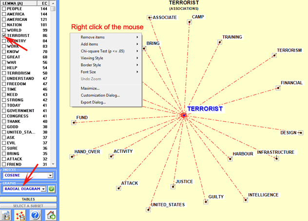
Each click on a item produces a new chart and, by using the right click of the mouse, it is possible to to open a dialog box which allows several customizations (see below).

Tables reporting various measures allow us to check the relationships between occurrences and co-occurrences concerning the words (up to 50) that are most associated to the target ones.

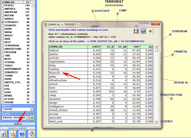
The reading keys are as follows:

· LEMMA (A) = selected lemma;
· LEMMA (B) = lemmas associated with LEMMA (A);
· COEFF = value of the selected index;
· TOT EC = total amount of elementary contexts (EC) or n-grams in the corpus or in the analysed subset;
· EC_A = total amount of EC that contains the selected lemma (A);
· EC_B = total amount of EC that contains every associated lemma (B);
· EC_AB = total amount of EC where lemmas "A" and "B" are associated (co-occurrences);
· CHI2 = chi square value concerning the co-occurrence signifiance;
· (p) = probability associated with the chi square value (def=1);

In the case of chi square test, for each couple of lemmas ("A" and B") the structure of the analysed table is the following:

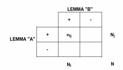
Where : nij = EC_AB; Nj = EC_A; Ni = EC_B; N = TOT EC.

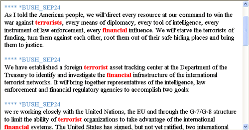
A click on each table item (e.g. 'financial') allows us to save a HTML file with all the elementary contexts (i.e. sentences or paragraphs) where the selected lemma co-occurs with the central word (e.g. 'financial' and 'terrorist').

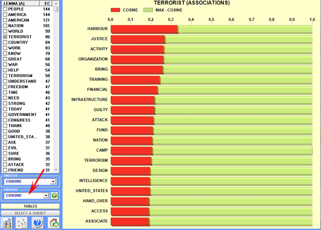
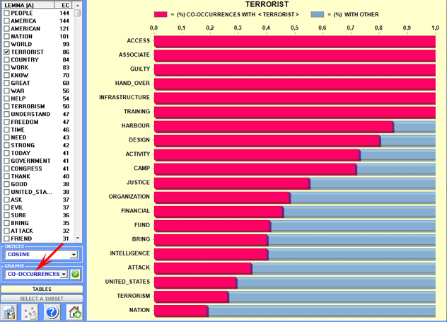
Further graphs (bar charts) allow us to appreciate the values of the coefficient used and the percentage of co-occurrence contexts (see below).

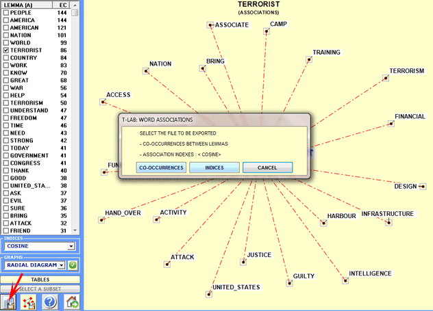
By clicking the button at the bottom left, the user can export various types of tables (see the picture below).

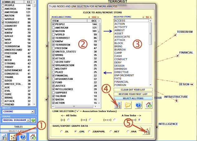
A specific T-LAB window (see the picture below) allows us to create various files which can be edited by software for network analysis (e.g. Gephi, Pajek, Ucinet, yEd and others). In this case the nodes are words associated with the target key-term; so each time it is possible to map the local network of such a term. The available options are the following: select the words (i.e. the 'nodes') to be inserted into the graph (see steps 2 and 3 below), export the corresponding adjacency matrix (see step 4 below), export the selected graphical file (see step 5 below).

N.B.: In T-LAB 10 the following window has been replaced by the Graph Maker tool.

For example, .gml files exported by T-LAB can allow us to create graphs like the following.

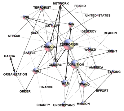
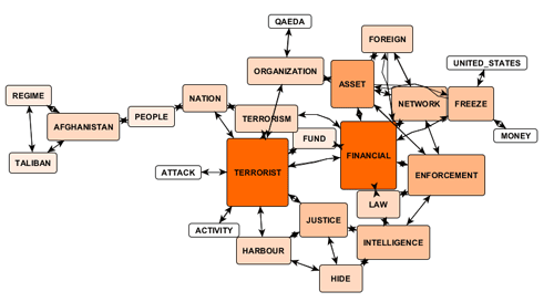
N.B.: The first of the above graphs has been created by means of Gephi (https://gephi.org/ ), the second by means of yEd (http://www.yworks.com/en/products_yed_download.html/ ), which both are available as free download.

The way T-LAB computes the association (or proximity) indexes is illustrated in the corresponding section of the Manual/Help (see the glossary). All these 'first order' indexes are obtained through a normalization of the co-occurrence values concerning word pairs; so, in such computation, two words which never co-occur have an association index equal to '0' (zero). Differently, the 'second order' indexes highlight similarity phenomena which are not directly related to co-occurrences between word pairs; in fact, in this case, two words which never co-occur can nevertheless have a high similarity index.

By making reference to structural linguistics, we could say that 'first order' indexes point out phenomena concerning the sintagmatic axis ('in praesentia' combination and proximity, i.e. each word 'near to' the other), whereas 'second order' indexes point out phenomena concerning the paradigmatic axis ('in absentia' association and similarity, i.e. quasi-synonymity between key-terms used within the same corpus).
In order to understand how T-LAB computes 'second order' similarities it is useful to recall that all 'first order' indexes can be gathered in proximity matrices like the following (Matrix 'A').

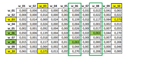
Matrix 'A' - First Order Similarities

In the above 'A' symmetric matrix the values in yellow (0.373) correspond to the highest 'first order' similarity between the selected words and indicate the association between words 'w_03' and 'w_10'. More specifically, 0.373 is an equivalence index obtained by dividing their squared co-occurrences by the product of their occurrences (360^2/627*553).
Starting from the above 'A' matrix, T-LAB builds a second matrix (see 'B' below) obtained by computing all cosine coefficients between all 'A' columns. For example, in matrix 'B' below the highest similarity index (the one in green: 0.905) has been obtained by computing the cosine coefficient between the corresponding columns of the 'A' matrix (i.e. w_06 and w_10), the 'first order' similarity of which is quite low (0.063).

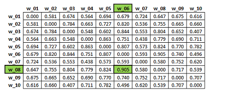
Matrix 'B' - Second Order Similarities

In other words, a 'first order' index is obtained by a formula which includes co-occurrence and occurrence values, whereas a 'second order' index is obtained by multiplying two normalized feature vectors.
Beyond any computational issue, we have to recall that in the above two cases ('A' and 'B' matrices) we are dealing with two very different phenomena. In fact, in the case of 'A' we are focusing on the co-occurrences between word pairs, whereas in the case of 'B' - and without any reference to their direct co-occurrences - we are focusing on the 'similarity' between feature vectors (see the matrix 'A' columns) which refers to the use (and so to the meaning) of the corresponding words.
For example, by analysing 'The Audacity of Hope' (i.e. a book written by B. Obama) it is possible to point out that - when using 'first order' measures - the word 'nuclear' is strongly associated with co-occurrent words like 'weapon', 'option', 'arms' etc.; whereas, when using 'second order' measures, 'nuclear' results strongly associated (i.e. similar) to 'destruction', even so the co-occurrence value of this word pair (i.e., 'nuclear' and 'destruction') is just '1' (one).

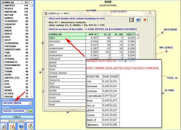
The tables shown by T-LAB allow the user to check both the second order similarities (see column SIM-II below) and the first order indexes (see column EQU-I, i.e. Equivalence Index). Moreover, by clicking any item of such a table, it is possible to generate HTML files which allow the user to check which features determine the similarity between each word pair. For example, the following table shows that the second order similarity between 'war' and 'figh' is - above all - determined by shared words like 'win', 'terrorism', etc..